How Neural Networks Learn: The Math Behind a Fast Prediction

TL;DR: A neural network is a parameterized function. Training measures the error with a loss, computes gradients with backpropagation, and updates the parameters with gradient descent. A low training loss is not the goal. Generalization to new data is. I use a laptop-price toy model with real numbers so the mechanism stays visible.

This is part 2 of a two-part series. Part 1 covers fast predictions versus deliberate investigation.

In part 1 I split decisions between a fast predictive model and a slower, deliberate process. This post goes one level down: how does a fast model get its behavior in the first place?

I’ll start with a model so small you can do the math by hand, then build up to neural-network training.

A model is a function with adjustable parameters

A conventional program follows relationships the developer writes down. A machine-learning model has numerical parameters that get adjusted using examples. The compact way to write it is ŷ = f(x; θ). Here x is the input, θ is the set of parameters, and ŷ is the prediction.

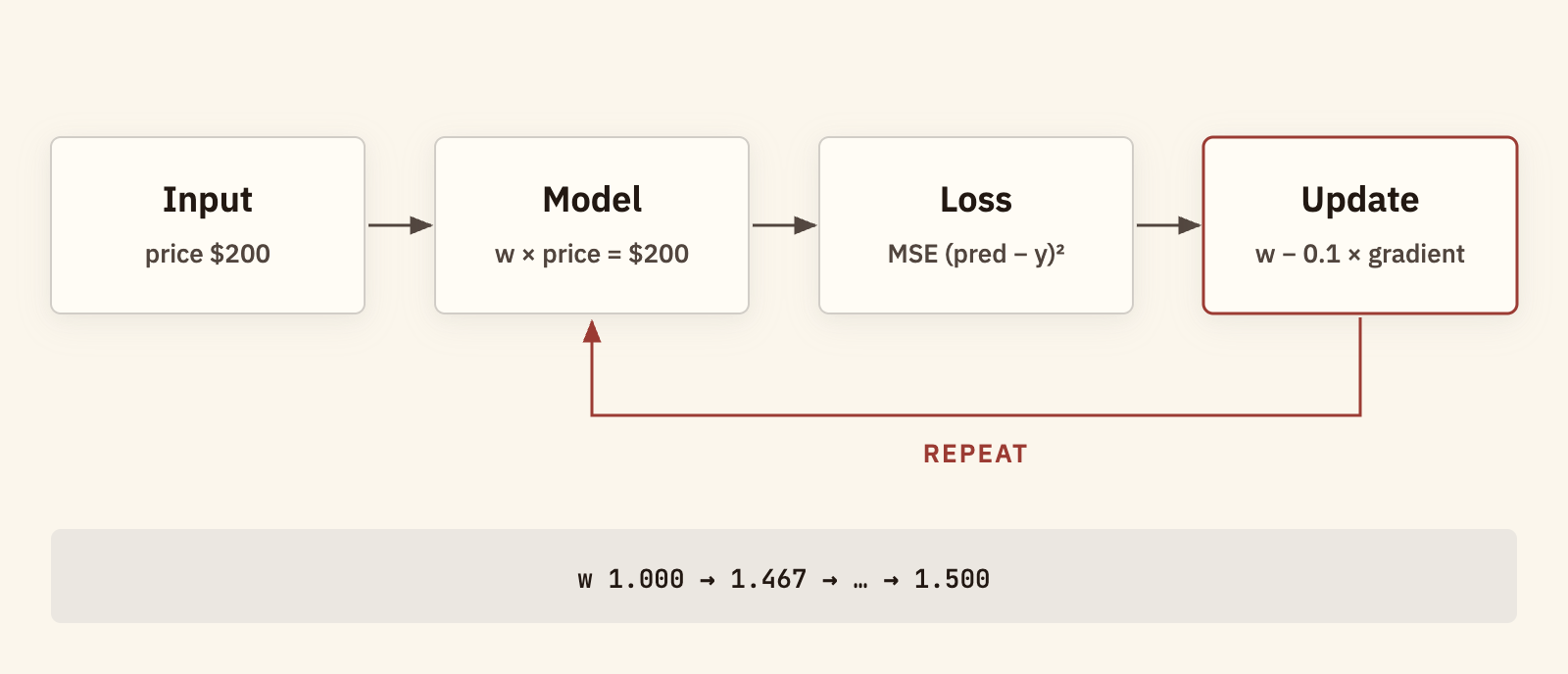
Say I want to predict a laptop’s resale price from its purchase price. I use a deliberately simple model: predicted resale price = weight × purchase price. A laptop bought for $200 that sells for $300 gives a target weight of 1.5 for that example. I initialize the weight to 1, so the model predicts $200. It is $100 off, and I need a way to measure that error and shrink it.

Loss: define what counts as an error

A loss function turns prediction errors into one number to minimize. For numerical predictions, mean squared error (MSE) averages the squared differences between predictions and targets:

MSE = (1/n) × Σ(ŷᵢ − yᵢ)²

Squaring keeps positive and negative errors from canceling, and it punishes large errors more.

The loss captures the training objective I chose. It does not capture every requirement of a production system. A low training loss does not guarantee good predictions when market conditions change.

Gradient descent: step toward lower loss

The gradient tells you how sensitive the loss is to each parameter, and in which direction. Gradient descent uses it to update each weight. In one dimension:

new weight = old weight − learning rate × gradient

Take the toy laptop dataset, with prices in hundreds of dollars: the pairs (1, 1.5), (2, 3), and (3, 4.5). The loss works out to L(w) = (14/3)(w − 1.5)². At w = 1, its derivative is about −4.667. With a learning rate of 0.1, the first update gives w ≈ 1.467. That is already very close to the target of 1.5.

The learning rate sets the step size. Too small and training is slow. Too large and it overshoots or diverges. Real optimizers build on these ideas with smarter update rules.

Backpropagation: gradients through many layers

A real network has many parameters spread over layers. In the forward pass, data flows through the model to produce a prediction and a loss. Backpropagation then applies the chain rule of calculus to work out how the loss changes with respect to the parameters, all the way back through the network. The optimizer uses those gradients to update the parameters.

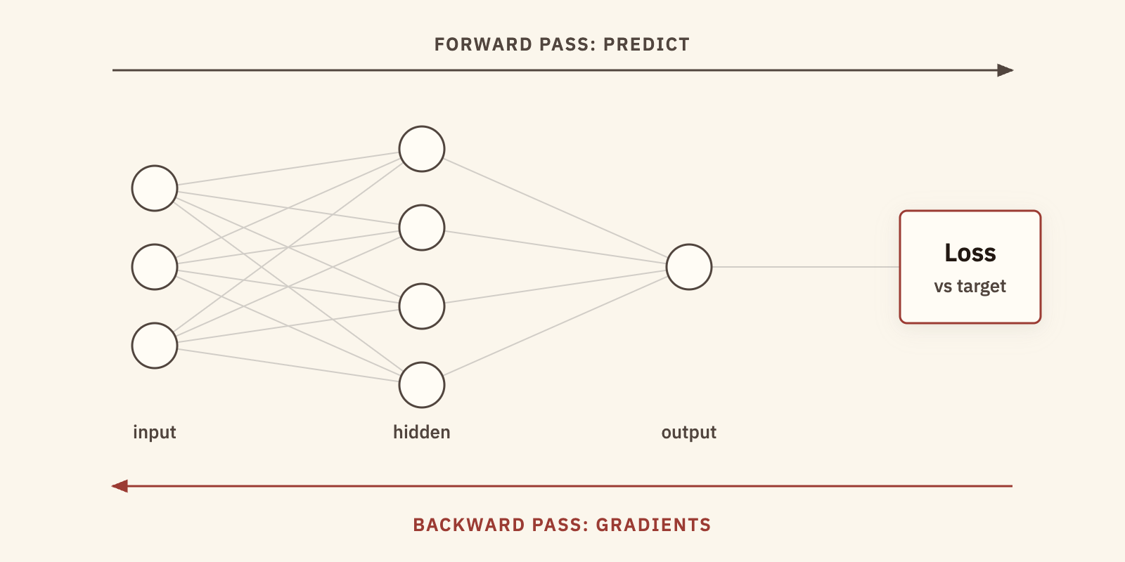
These are two different operations. Backpropagation computes gradients. Gradient descent, or another optimizer, performs the update. Libraries like PyTorch automate the differentiation, and the mechanism underneath stays the same.

A minimal training iteration looks like this:

prediction = model(inputs)
loss = loss_function(prediction, targets)
optimizer.zero_grad()
loss.backward()
optimizer.step()

Training updates the model’s parameters. Ordinary inference applies the learned parameters to new inputs and updates nothing.

Overfitting: a low training loss can mislead

Suppose a resale-price model predicts historical laptops almost perfectly but does badly on newly listed ones. It may have learned quirks of its training sample instead of a relationship that holds up. That is overfitting.

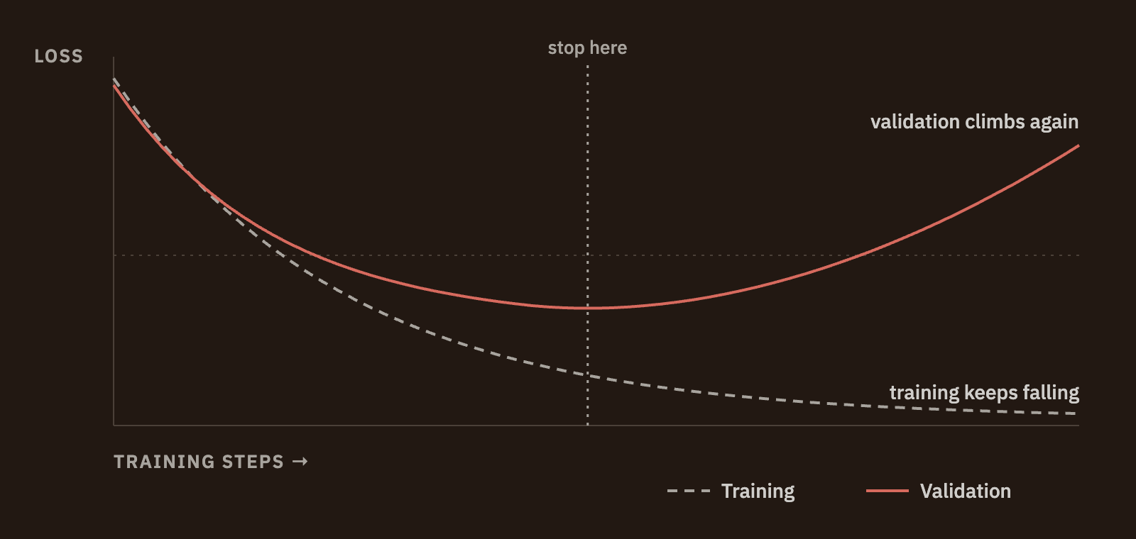
To check generalization, I keep separate training, validation, and test sets. Training data updates the parameters. Validation data helps me pick architectures and hyperparameters, and decide when to stop. A held-out test set estimates the final performance. For prices that change over time, a chronological split can tell you more than randomly mixing old and new transactions.

Early stopping, regularization, representative data, and a model of the right size all help. None of them removes the need for realistic evaluation.

Back to System 1 and System 2

Training can spend a lot of computation learning a mapping. Inference then applies it fast. That makes specialized predictive models a good fit for repeated, well-defined tasks. But a fast model can fail on unfamiliar inputs, and it can be confidently wrong. The process around it may need to fetch new evidence, apply safety rules, or escalate to a person.

Producing a score and deciding what action that score justifies are different jobs.

Run it yourself

Here is the whole toy example in plain Python, with no ML dependencies, so the learning mechanism stays visible. Save it as train_model.py and run it with Python 3. It isn’t published anywhere else on this site.

# Basic gradient descent: prices expressed in hundreds of dollars.
data = [(1.0, 1.5), (2.0, 3.0), (3.0, 4.5)]
weight = 1.0
learning_rate = 0.1
for epoch in range(20):
    loss = sum((weight*x-y)**2 for x,y in data)/len(data)
    gradient = sum(2*(weight*x-y)*x for x,y in data)/len(data)
    weight -= learning_rate*gradient
    print(f"epoch={epoch+1:02d} loss={loss:.6f} weight={weight:.6f}")
print(f"Predicted resale for $400 purchase: ${weight*400:.2f}")

Watch the weight approach 1.5. Then try learning rates of 0.001 and 0.5. When I ran it, 0.001 only got the weight to about 1.09 after 20 epochs, and 0.5 overshot further on every step until the weight was around −10¹¹.

Where I land

A neural network is a parameterized mathematical function. Training measures errors, computes gradients, and updates parameters to improve predictions. What decides whether those predictions are useful is how well they generalize to new data, not how well they fit the training set.